Details
Modeling Levels
PRAM supports modeling on three levels of abstraction: Domain, class, and rule. Apart from being flexible, this design choice delivers expressive brevity in that it allows the modeler to invoke models in a space- and time-efficient manner. In what follows, we briefly describe an example model and then demonstrate how that model can be implemented on each of the three level.
The SIRS Model
The SIR epidemiological model 1 will help us illustrate the different modeling levels. In that model, population is compartmentalized into susceptible (S), infectious (I), and recovered (R). As shown on the image below, an infectious disease is transmitted between susceptible hosts with the rate β who eventually recover with rate γ. Because getting a disease does not need to result in life-long immunity to it, the model can be augmented by allowing recovered hosts to become susceptible again with rate α (which results in the SIRS model).
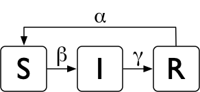
The SIRS model
The Domain Level
The domain level allows the modeler to express their models on the level of their research area. For example, being familiar with the different models of infectious diseases, it would be natural for an epidemiologist to invoke a model like the SIRS directly. Here is a Python example of just that:
SIRSModel('flu', β=0.05, γ=0.50, α=0.10)
The Class Level
A modeler can also work on the class-of-models level. For example, an epidemiologist may know that the SIRS model can be implemented as a time-invariant Markov chain. Here is an example of how that can be coded in the PyPRAM package using the TimeInvMarkovChain rule:
β, γ, α = 0.05, 0.50, 0.10
transition_matrix = {
    's': [1 - β,     β,  0.00],
    'i': [ 0.00, 1 - γ,     γ],
    'r': [    α,  0.00, 1 – α]
}
TimeInvMarkovChain('flu', transition_matrix)
The Rule Level
Finally, a modeler may choose to descend to the lowest level and implement the dynamics of their model directly. This is beneficial if what they are trying to express diverges from the set of modeling classes PyPRAM provides (or to encode a particular sort of interaction between different models). Extending an existing class (e.g., the TimeInvMarkovChain) is an example of modeling on the rule level as well even if minimal portions of the model dynamics are overridden. Here is a pseudo-code for the (slightly extended) SIRS model:
rule_flu_progression():
    if group.feature.flu == 's':
        p_inf = n@_{feature.flu == 'i'} / n@    # n@ - count at the group's location
        dm     p_inf -> F:flu = 'i', F:mood = 'annoyed'
        nc 1 - p_inf
    if group.feature.flu == 'i':
        dm 0.2 -> F:flu = 'r', F:mood = 'happy'
        dm 0.5 -> F:flu = 'i', F:mood = 'bored'
        dm 0.3 -> F:flu = 'i', F:mood = 'annoyed'
    if group.feature.flu == 'r':
        dm 0.1 -> F:flu = 's'    # dm - distribute mass
        nc 0.9                   # nc - no change

rule_flu_location():
    if group.feature.flu == 'i':
        if group.feature.income == 'l':
            dm 0.1 -> R:@ = group.rel.home
            nc 0.9
        if group.feature.income == 'm':
            dm 0.6 -> R:@ = group.rel.home
            nc 0.4
    if group.feature.flu == 'r':
      dm 0.8 -> R:@ = group.rel.school
      nc 0.2
This pseudo-code is based on a Python-like notation we have been working on to help to expose the internal workings of a model without resorting to often unnecessarily verbose Python source code.
Ordinary Differential Equations
Mass Space
PyPRAM supports simulating systems of ordinary differential equations (ODEs) operating on three types of spaces. First, systems of ODEs can be used as mass conversion operators. For example, the image below shows the conversion of mass for two substances, A and B, described by the exponential decay equation (i.e., \(dN/dt = -\lambda N\)). The decay constants for the two substances are \(\lambda_A = 1\) and \(\lambda_B = 0.05\).
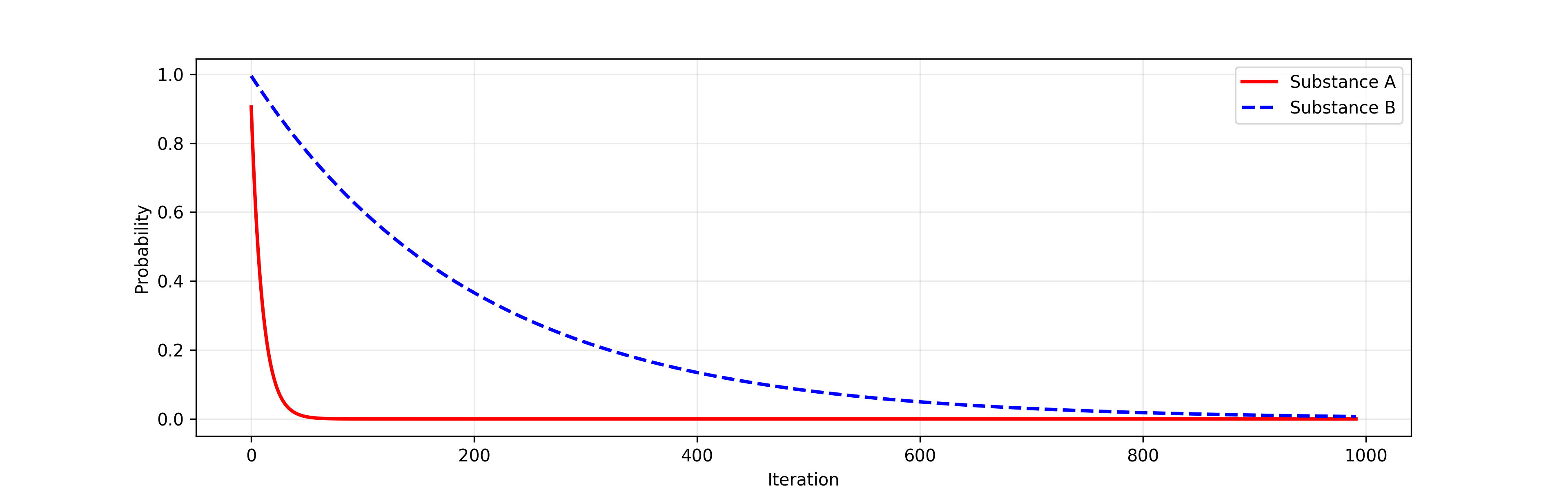
Exponential decay of two substances
As another example, the time series below shows the result of simulating a system of ODEs describing the SIR model.
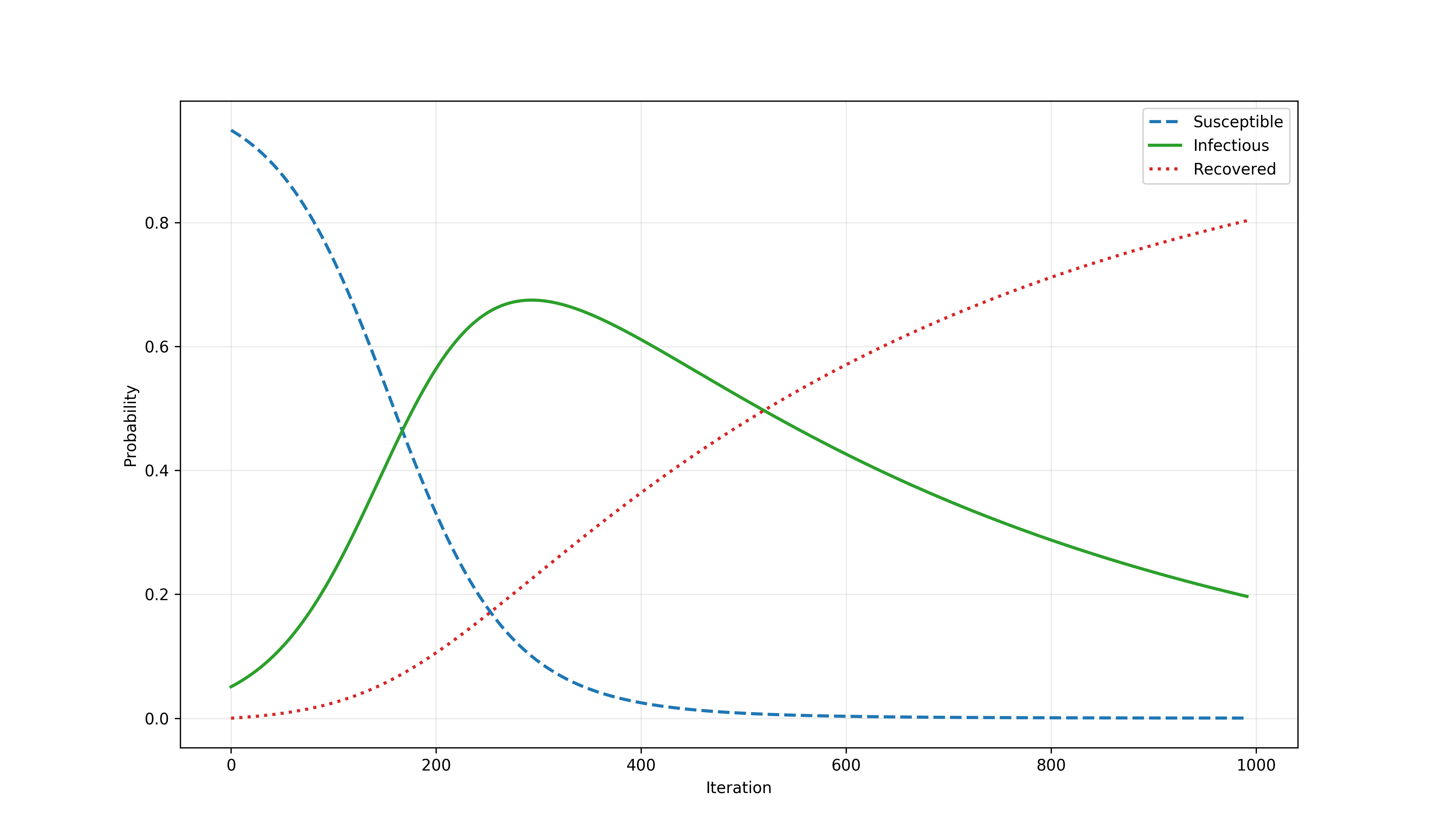
The SIR model
Group Space
The second space which can be affected by a system of ODEs is given by groups. Because groups are defined by the values of their attributes and relations, this results in mass conversion (or flow) between groups, but the machanism by which this occurs is different than when the ODEs operate on the mass space.
The time series below shows the result of simulating the Lotka-Volterra population dynamics model. That model expresses the cyclic relationship between the size of prey population that grows via reproduction and the size of predator population which grows by consuming the prey.
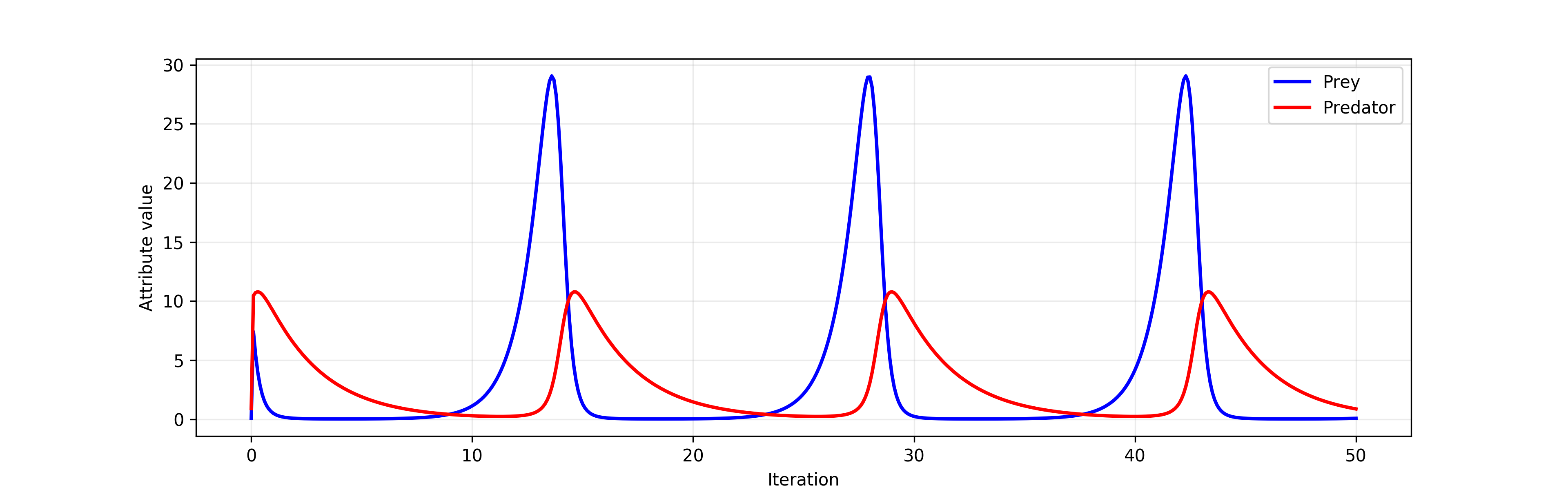
The Lotka-Volterra model
Rule Space
Finally, the numeric integrator for a system of ODEs can be kept internal to the PRAM rule. In that case, it does not interact with the simulation context directly. Nevertheless, the results of the integration are available to all other rules. For example, the image below shows the phase plot of atmospheric convection modeled with three ODEs that form the Lorenz system. The solution to this particular initial value problem is the Lorenz attractor.
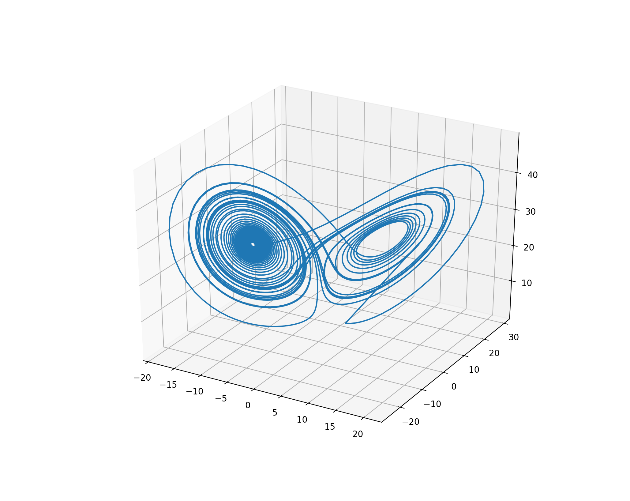
The Lorenz system
Composite Simulations
One of the goals of PyPRAM is to elucidate the interactions between complex systems. The package hopes to do that via composite simulations, i.e., simulations composed of different models which are allowed to work independently and interact by simultaneously changing the shared simulation state space.
The SIR Model with a Flu-Spike Event
The time series below is a result of a simulation combining the SIR model with an event (i.e., a time-point perturbation). That event converts a large proportion (specifically, 80%) of the recovered agents back into susceptible.

The SIR model with an event
The SIR Model with a Flu-Spike Process
A more interesting and realistic scenario might involve not an event but a process (i.e, a time-span perturbation). For example, the time series below shows the intensity of a process described by the scaled gamma distribution.
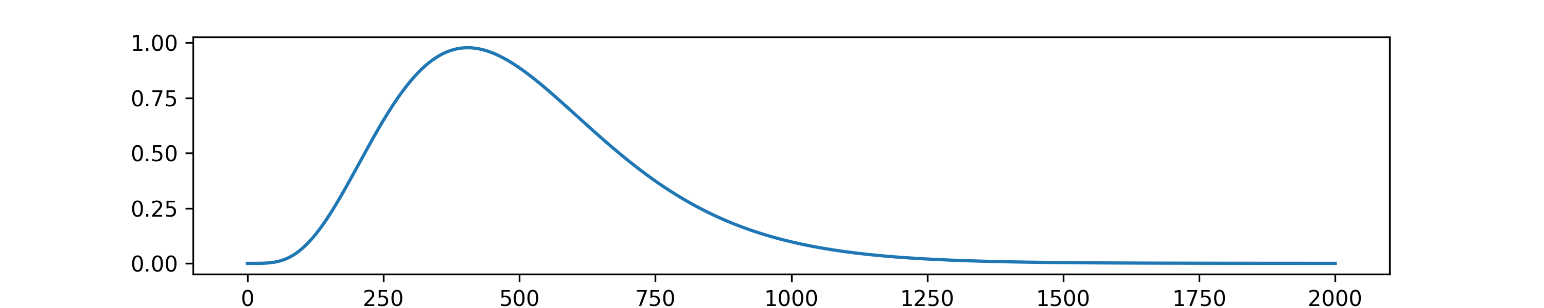
The gamma process
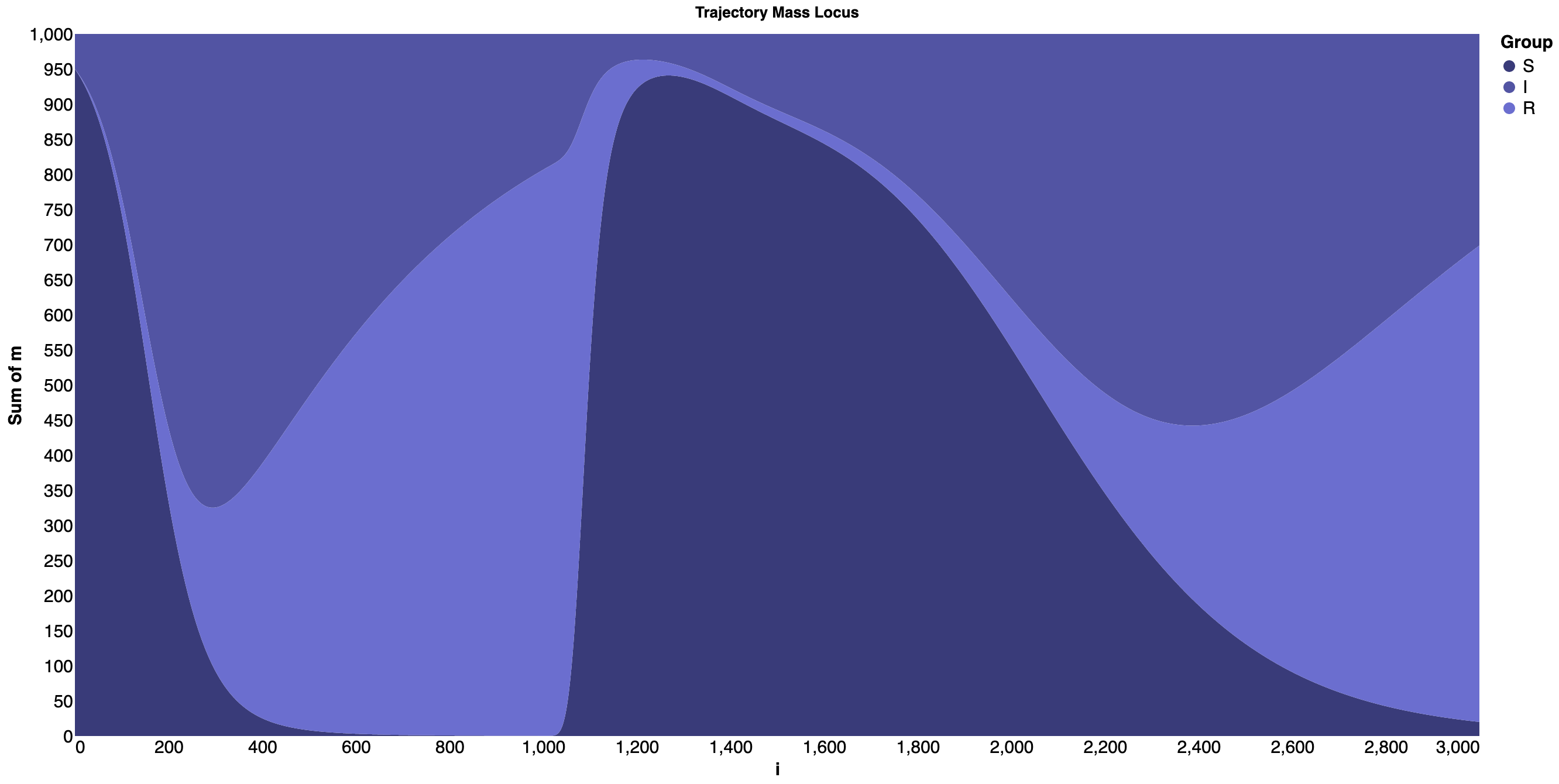
When this gamma process is combined with the SIR model, the PRAM simulation produces a time series shown on the image below. Iterations 1-999 are dominated by the SIR model which converts mass from S to R via I (i.e., susceptible to recovered via infectious). However, from that point on (i.e., for iterations of 1000-3000), additionally to that model, the gamma process shown above converts a portion of the recovered agents back into susceptible. As shown on the plot below, the interplay of the two PRAM rules (with the SIR model dynamics being encoded by a system of ODEs) produces an interesting effect of the infection level in the population being stretched in time plausibly resulting in a model of a long-term epidemic.
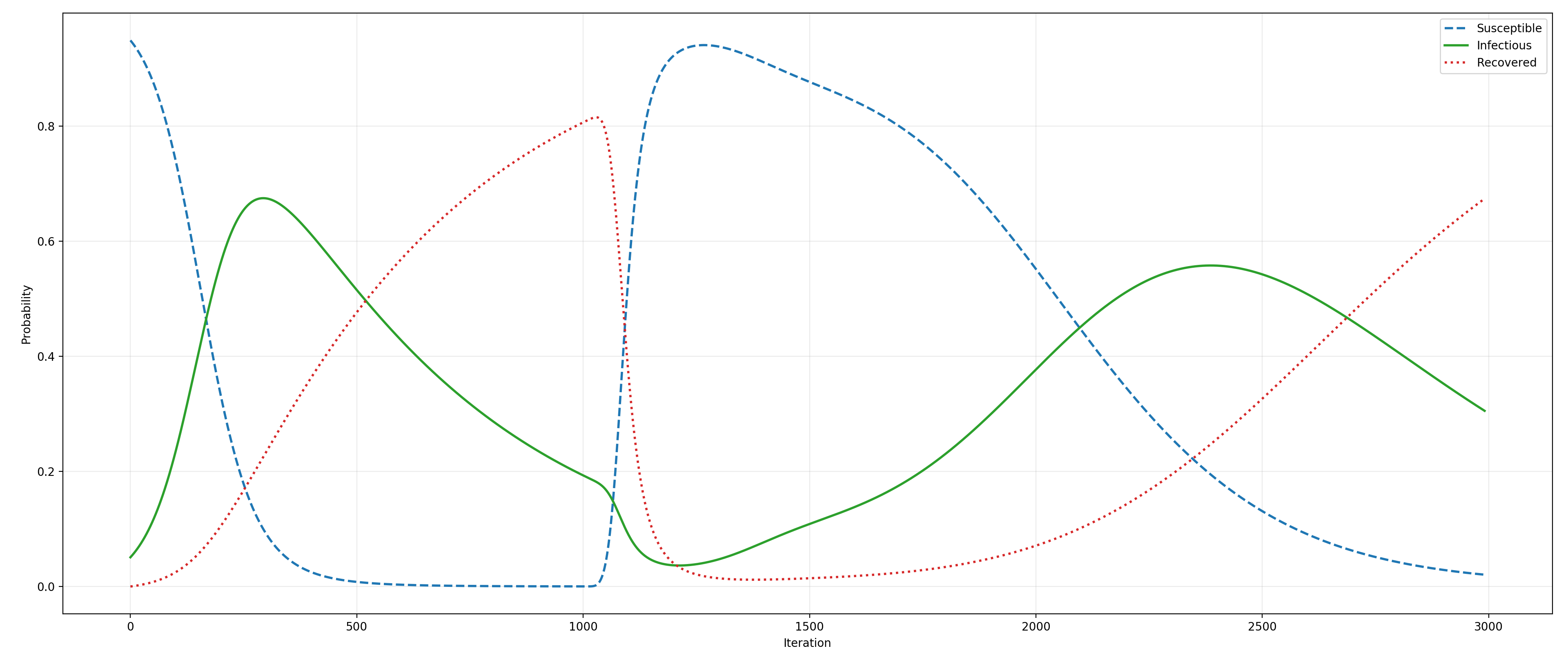
The SIR model with a gamma process
The Lotka-Volterra Model with a Food Restriction Process
The Lotka-Volterra model of population dynamics contains four parameters. When one of them, the prey reproduction rate parameter, is affected by a linear process that decreases it slowly but surely, the following picture emerges.
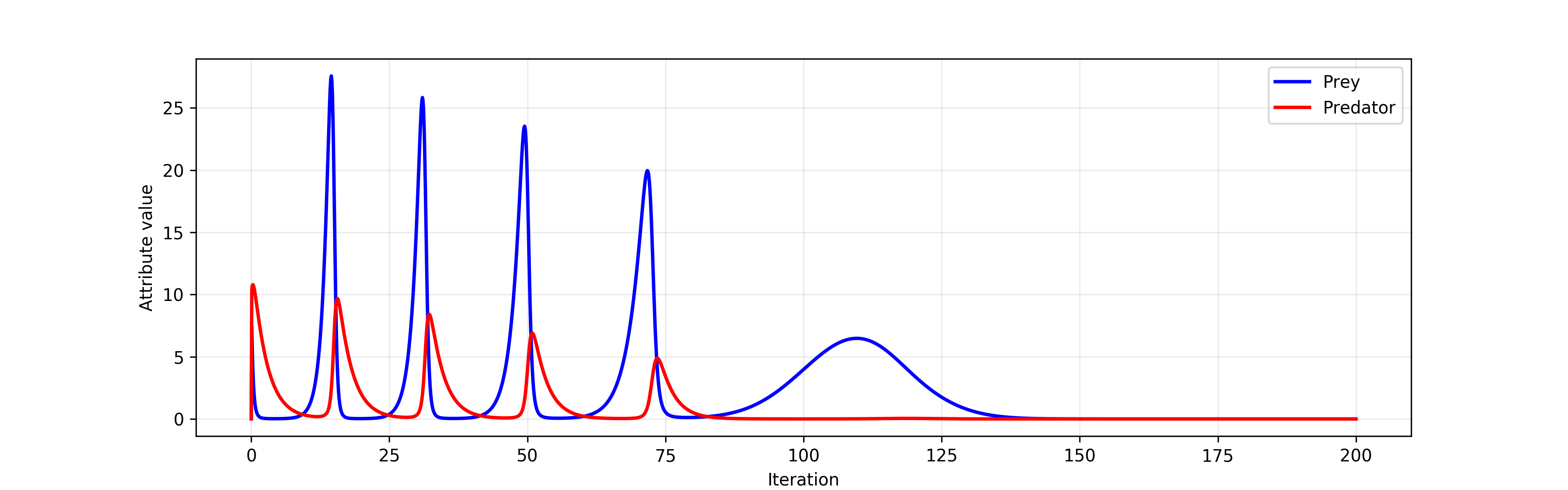
The Lotka-Volterra model with a linear process
By decreasing the reproductive rate of prey, that linear process models increasingly hostile natural environment. The process does not directly disturb the sizes of the two populations and affects the population dynamics indirectly (plausibly by restricting the prey food sources). While using such a simple process is perfect for expositionary purposes, a more realistic model would involve breaking the linear process down into sub-processes, each corresponding to the dynamics of an asymptotically barren ecosystem.
Even though the process changes the prey reproductive parameter in very small decrements, it nevertheless leads to the eventual extinction of the predator population (due to insufficient size of the prey population) and then the prey population itself. If we assume that the simulation parameters are biologically and ecologically valid, this simulation predicts the predator species to go extinct in 80 years and the prey population to follow in another 50 years.
Mass Dynamics
In the context of a PRAM simulation, mass dynamics can be defined in at least three related but distinct ways. First, we could understand it as mass locus (\(m\)); such conceptualization would allows us to answer the question “Where is mass?” Second, we could define it as mass flow (i.e., the first derivative of mass locus, \(dm/dt\)) which would permit answers to the question “How did it get there?” Finally, we could talk of the mass flux (or rate of mass flow, i.e., first derivative of mass transfer and the second derivative of mass locus, \(d^2m/dt\)). The rate answers the question “How quickly did it move?”
Mass Spaces
Mass dynamics in PRAMs can be considered in the group space or the probe space. The group mass space is a partition defined by group attributes and relations and thus contains all the groups in a simulation (for that reason, the name simulation mass space would be adequate as well). The probe mass space on the other hand is typically smaller (i.e., it has fewer dimensions) because the mass distributed among the groups is typically aggregated by probes. For example, while the SIR model can be invoked in a simulation containing many agents attending many schools, a probe defined by the user will reveal their interest to be on a high level of, e.g., “size of populations of infected students at low vs medium income schools over time.”
Mass Locus
Below are a few examples of how mass locus can be visualized using steamgraphs. First, we have the SIR model which was described earlier.

Streamgraph for the SIR model
Next, we have a simulation of the SIR model composed with a gamma process which at iteration 1000 starts to convert recovered agents back into susceptible. That gamma process quickly overpowers the SIR model’s attempts to convert agents into recovered (via infectious) but then eases off and eventually play no role.
Streamgraph for the SIR model and a gamma process
Next, we have the segregation model 2 in which mass dynamics is the result of the agents’ motivation to be close to other similar agents (e.g., blue agents want to be in proximity of other blue agents) and far away from dissimilar agents (e.g., blue agents do not want to congregate near red agents).

Streamgraph for the segregation model
Finally, we have a simulation of the SIR model at eight different schools. The SIR models at each of those schools are slightly different in that the transmission probability depends on the size of the school, i.e., the probability of a student to become infected is proportional to the number of infectious students around him. In that way, larger schools are more likely to be afflicted by an epidemic.
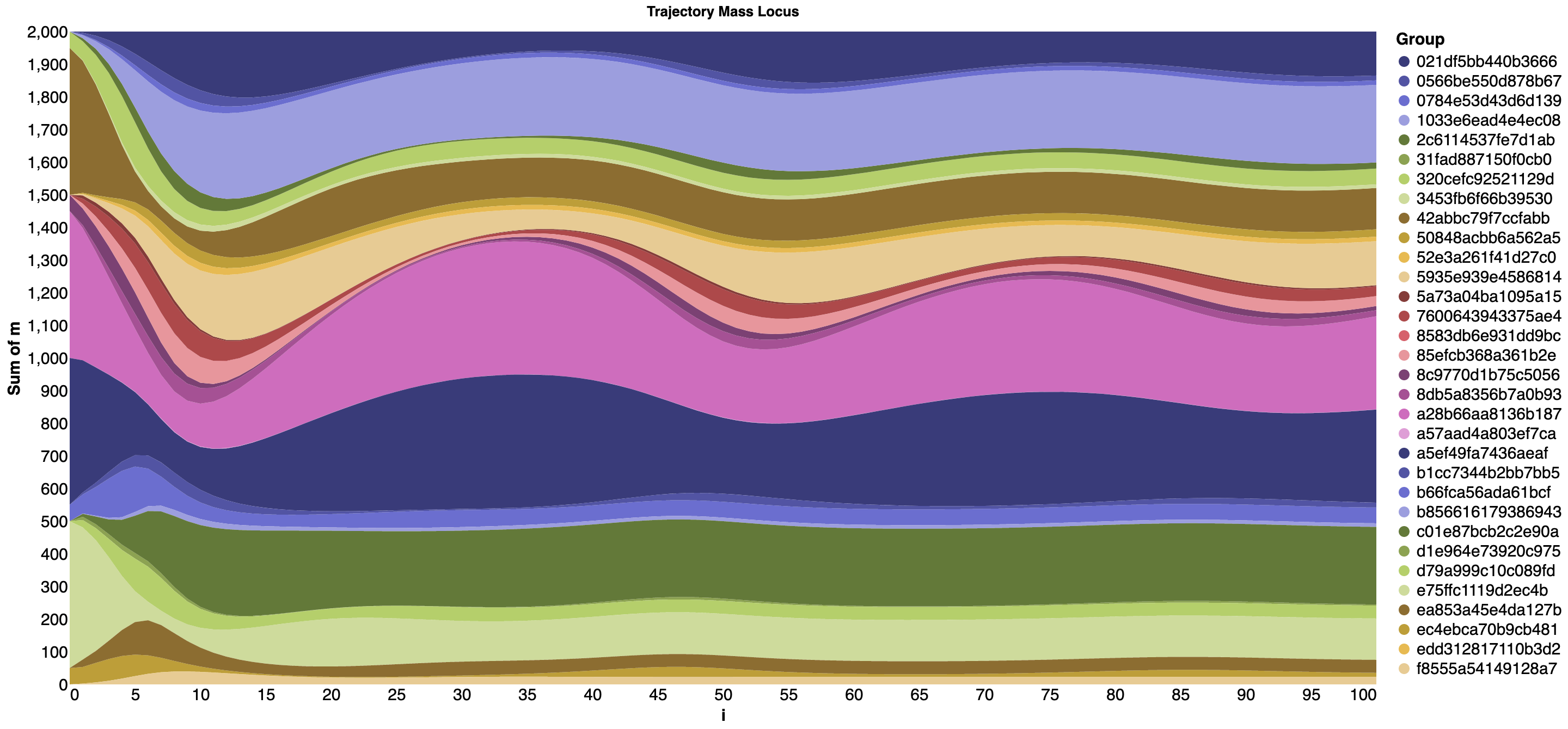
Streamgraph for the eight-schools simulation
Mass Flow
Below is an example of visualization of mass flow in the SIR model that has been run for seven iterations.

Trajectories and Trajectory Ensembles
A PRAM simulation need not to be deterministic. In fact, simulations imbued with stochasticity are likely the more interesting kind. In order to properly account for a stochastic nature of those simulations, the software enables execution of multiple independent simulations. The trace of those simulation runs yields an ensemble distribution which can then be inspected statistically for patterns (e.g., the expected number of years until underground water wells dry up in a region given water utilization strategies S1 versus S2 or the worst-case scenario under a set of utilization strategies). Because the states of individual simulations can be conceived as sequential interacting samples of the system state, this method belongs to the mean field particle class. While beginning with a set of user-defined or random initial states (or a combination thereof) is the simplest solution, a more elaborate initial state selection could be employed as well.
Example: The SIRS Model + Beta Perturbation
Let us illustrate this idea with a simulation of two interacting models. The first model is the SIRS model. The second model is a stochastic process that at every simulation step converts a small portion of the recovered agents back into susceptible. That random conversion probability is a random draw from the \(\text{Beta}(2,25)\) distribution. Below is the histogram of 100,000 such draws.
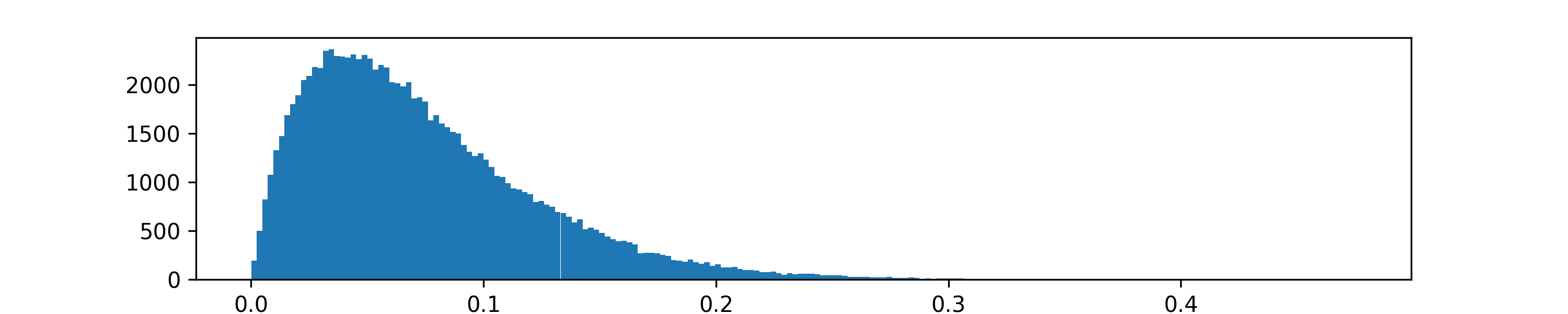
Beta distribution
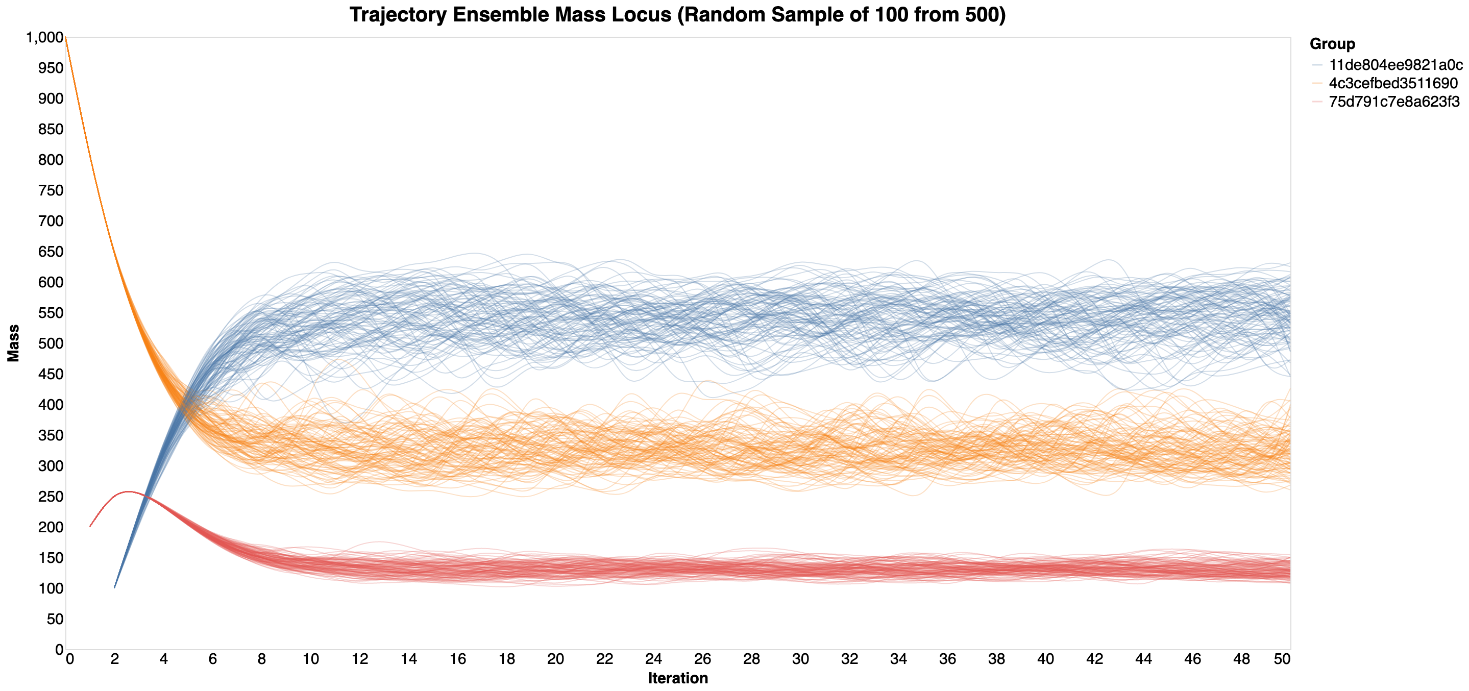
While the result of these two models interacting is fairly easy to anticipate, this may not be the case for larger systems of models. Below is a line plot of 10 randomly selected trajectories of this ensemble. Note that the actual data is not smooth; the plot represents splines fitted to each of the three series within each of the 10 trajectories.
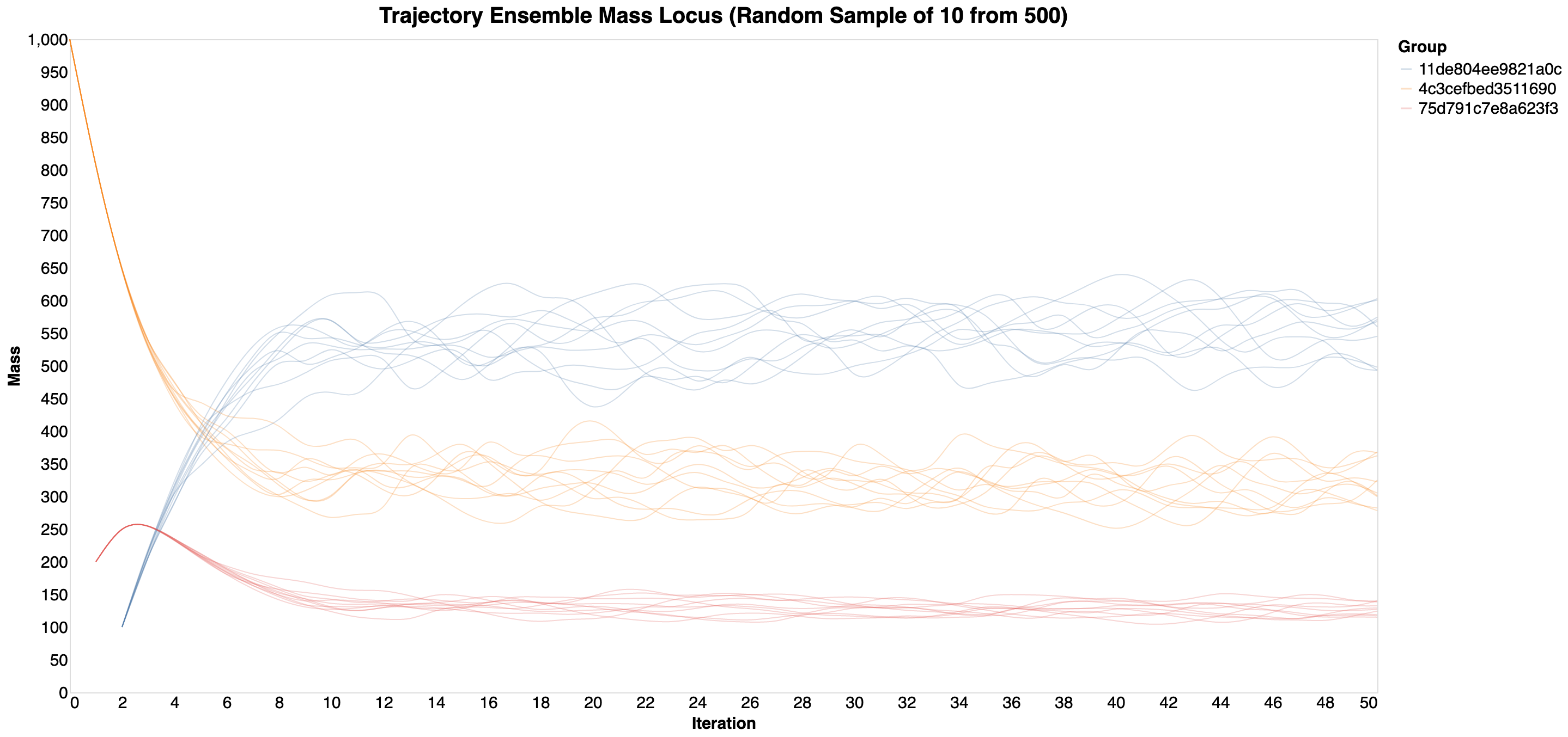
This is how a 100 samples would look like.
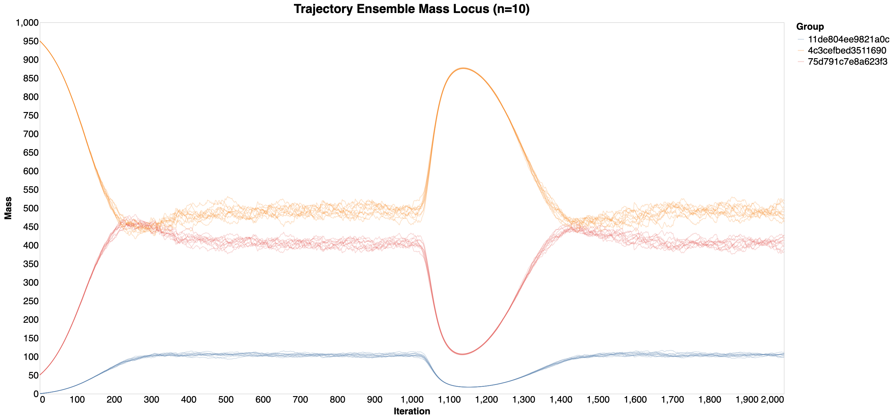
Example: The SIRS Model + Beta Perturbation + Gamma Process
In this example, we will investigate a simulation consisting of the same SIRS model and a beta perturbation but this time there will also be a gamma process which, like before, converts an increasingly large number of recovered agents into the susceptible ones only to ease off and eventually cease to affect the simulation altogether. Below is mass dynamics for an ensemble of 10 trajectories.
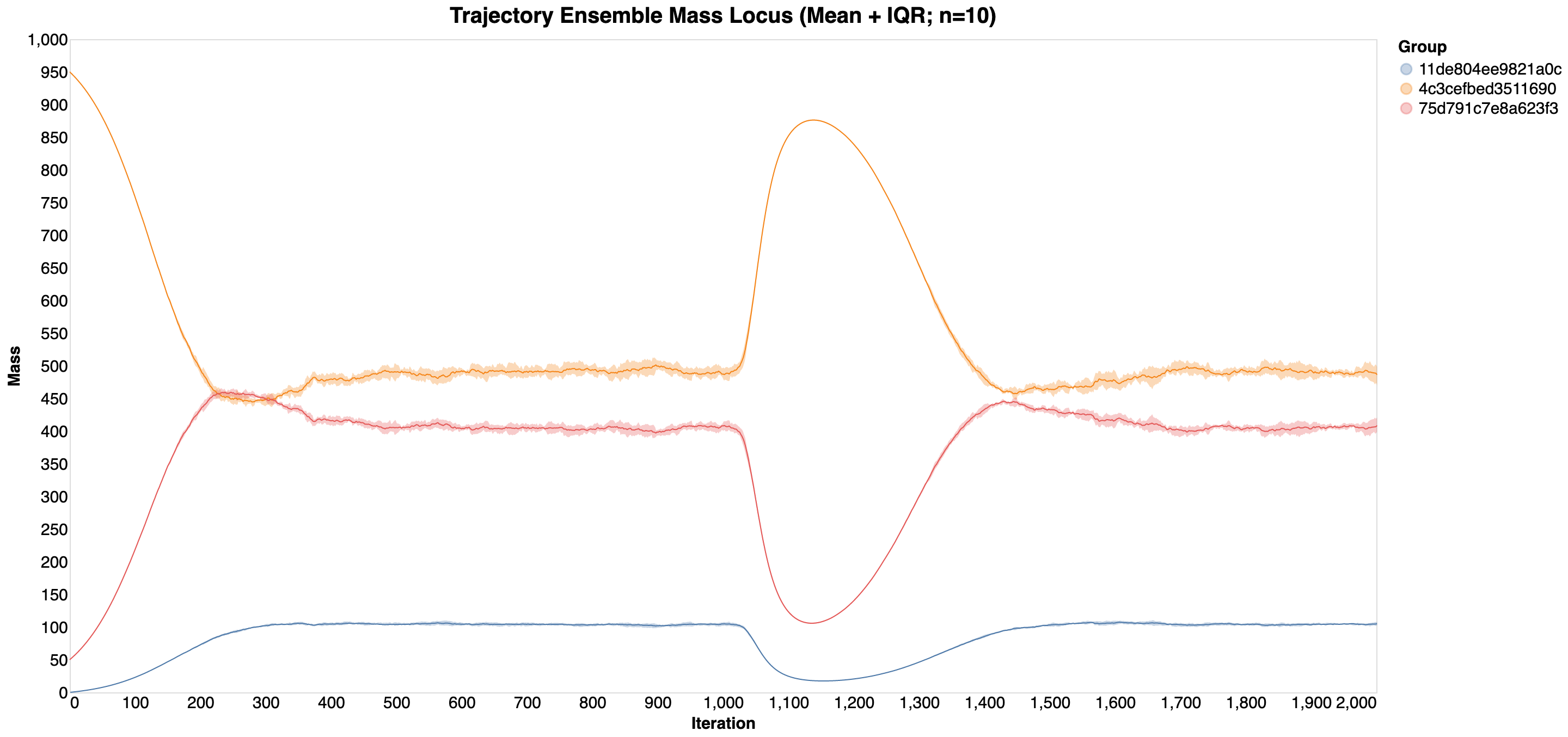
Because directly plotting large number of individual trajectories may not produce a clear image, trajectories can be aggregated over. One example of such aggregation is shown below. Here, the mean and the interquartile range (IQR) for each of the three groups (i.e., S, I, and R) is shown instead of the individual series.
References